Monte Carlo Path Tracing

You may understand the fundamental concept of light path tracing and why we often use Monte Carlo integration for it after reading this post. # Introduction

This is my note of a chapter "Path Integral Formulation of Light Transport" of Recent Advances in Light Transport Simulation: Theory & Practice, in SIGGRAPH 2013. I think the course is helpful for beginners to form a clearer picture about light path tracing.

Most images and some quotes in this post come from the slides of the course. The original author owns the copyright of them without a doubt.

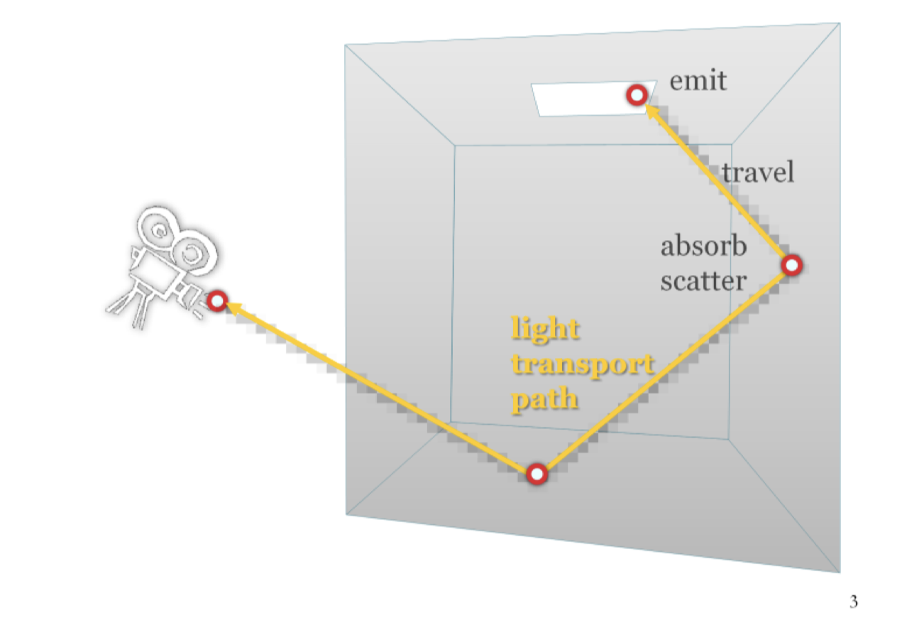
In physical world, the light is emitted from light sources, such as lamps. After reflection, refraction or absorption in the environment, the light could be seen only if it finally reached our eyes (or the camera in the picture). It may be natural to come up with the idea of formulating the process by calculating every ray emitted after defining surface attribute. However, it will result in computation of numerous invisible light, which refers to one that do not reach your eyes, and causes the waste of resources. Fortunately, we could simply reverse the process: emit the light from the eyes, so we will only need to calculate the light that matters. It is absolutely correct due to the phyisical knowledge that light path is reversible.

Now, let's get a further step. Try to imagine there are some objects in a house with a single window and you're standing outside. You are not allowed to get into the house but you want to see what's in the house, so you can only see them through the window. Apparently, your view is limited due to the window is not infinitely large.

Ok, and then we replace the words. The window is the screen, you are the observer (or the "camera"), and the objects compose a scene. As I mentioned above, we do path tracing in a reversed way in comparison to real world. In the illustration, the light pass inside (scene) through the window (screen) and then reach your eyes (camera). So its mirror turn should be "emitting lights from the camera through screen to the scene". To be more specific, as the screen is composed of limited pixels, we can descibe the process as emitting lights from the camera through each pixel of the screen to the scene.

This is the most fundamental idea about path tracing. And I will explain later how can we create a beatiful picture with this simple concept.

Path Integral Formulation

Programming is a concise art, and it is hard to solve a question without formal definitions. Path tracing is not an excepction. So let's first take a look at its mathematical term, which will help you understand why Monte Carlo is crucial.

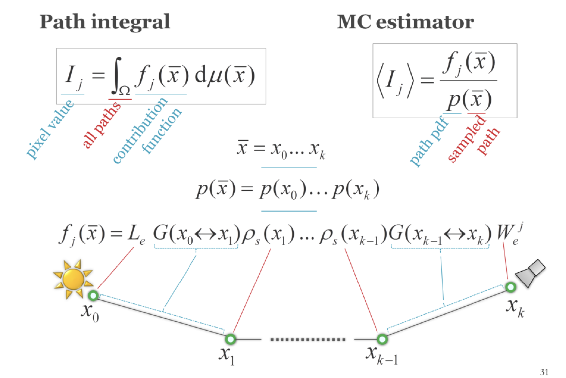
The picture above shows what a camera sees from a pixel: a collection of lights the reached to the pixel. Now we can define the camera response (the synthesis value of the pixel) in this term: \[ I_j = \int_\Omega f_j(\bar x)d\mu(\bar x) \]

The formula is called Path Integral Formulation, and its meaning is:

1. \(I_j\): the value of pixel j
2. \(\Omega\): all possible light paths
3. \(f_j(\bar x)\): measurement contribution function

Well, then what's "measurement contribution function" and what's \(\bar x\)? See the lecturer's first.

The measurement contribution function of a given path encompasses the “amount” of light emitted along the path, the light carrying capacity of the path, and the sensitivity of the sensor to light brought along the path.

Then this is the formal definition of \(f(\bar x), \bar x\): \[ \bar x = x_0x_1\cdots x_k \\ f_j(\bar x) = L_e(x_0 \rightarrow x_1)T(\bar x)W_e^j(x_{k-1}\rightarrow x_k) \] This picture shows what \(\bar x\) and \(T(\bar x)\) mean clearer:

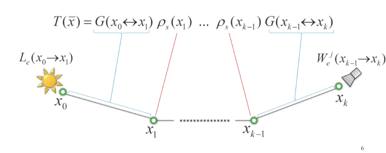
Now, let's try to understand the formula. First of all, a light transport path is a polyline with vertices corresponding to light scattering on surfaces. Like points on surfaces of walls, tables and desks.

1. \(x_i\): The i-th vertex

2. \(\bar x\): All vertices along the path

3. \(L_e(x_0 \rightarrow x_1)\): Emitted radiance. As we call the light resource \(x_0\), it can be understood as the light intensity of the source.

4. \(W_e^j(x_{k-1}\rightarrow x_k)\): Sensor sensitivity (or Emitted Importance). It depends on the distance or angle to the pixel, material feature, etc.

5. \(T(\bar x)\): Pass throughput. It is defined as the product of the geometric G and scattering terms associated with the path edges and interior vertices, respectively

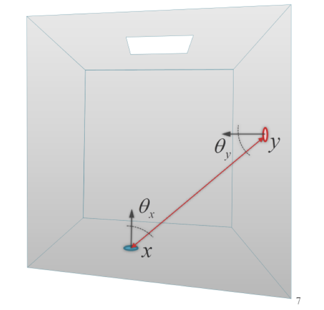
6. \(G(x\leftrightarrow y)\): Geometry term (or point-to-point form factor) of a path edge expresses the throughput of the edge due to geometry configuration of the scene. \[ G(x\leftrightarrow y) = \frac{|cos\theta_x||cos\theta_y|}{\|x-y\|^2}V(x\leftrightarrow y) \]

   

7. \(\rho_s(x_i)\): It is a abstract expression that means the value of each vertex, which may depend on material.

Now, let's read the integral again: \[ I_j = \int_\Omega f_j(\bar x)d\mu(\bar x) \] Oh yes, you understand it now! But wait, can you tell what "all paths (\(\Omega\))" mean?

Though it looks like a simple integral, there are infinite light paths and thus we cannot integrate \(\Omega\) directly. It can be rewritten as: \[ I_j = \sum_{k=1}^\infty \int_{M^{k+1}}f_j(x_0\cdots x_k)dA(x_0)\cdots dA(x_k) \] See it, the path integral actually hides an infinite sum over all possible path lengths.

Each summand of this sum is a multiple integral, where we integrate the path contribution over all possible positions of the path vertices. So each of the integrals is taken over the Cartesian product of the surface of the scene with itself, taken k+1 times (=number of vertices for a length-k path.) The integration measure is the area-product measure, i.e. the natural surface area, raised to the power of k+1.

As we all know, the computer is not good at dealing with infinity even if it is a simple form of integral. Thus, we need to find a method to numerically calculate the integral to get the value of each pixel.

Welcom Monte Carlo.

Monte Carlo Integration

Monte Carlo is a famous concept, if you have learned possibility theory or traditional machine learning methods you should be familiar with it.

If you didn't learn Monte Carlo before, let's take a quick look.

Suppose we are given a real function \(f(x)\) and want to compute the integral \(\int f(x) dx\) over some domain. The Monte Carlo integration procedure consists in generating a ‘sample’, that is, a random x-value from the integration domain, drawn from some probability distribution with probability density p(x). In the case of path integral, the xvalue is an entire light transport path.

For this sample \(x_i\), we evaluate the integrand \(f(x_i)\), and the probability density \(p(x_i)\). The ratio \(\frac{f(x_i)}{p(x_i)}\) is an estimator of the integrand. To make the estimator more accurate (i.e. to reduce its variance) we repeat the procedure for a number of random samples \(x_1 , x_2 , …, x_N\), and average the result as shown in the formula. This procedure provides an unbiased estimator of the integrand, which means that “on average”, it produces the correct result i.e. the integral that we want to compute.

The most well-known example of this method is estimating the value of \(\pi\) by throwing stones to a circle again and again. If you want to learn more about it or confused by unbiased estimator, try to find a statistical textbook.

Suppose you understood everything mentioned yet, let's see how to apply Monte Carlo integration to path tracing.

We can rewrite the Monte Carlo estimator of path integral formula first: \[ \langle I_j\rangle = \frac{f_j(\bar x)}{p(\bar x)} \] Now, for each pixel \(j\) we can apply Mote Carlo inegration by these steps:

1. Generate a random light transport path \(x\) in the scene.
2. Evaluate the probability density \(p(\bar x)\) of the path and the contribution function.
3. Evaluate the integrand \(f_j(\bar x)\).

Path Sampling

We already knew how to calculate \(f_j(\bar x)\), so now the question left is the path sampling method and its induced path probability density function (PDF) \(p(\bar x)\).

In fact, from the point of view of the path integral formulation, the only difference between many light transport simulation algorithms are the employed path sampling techniques and their PDFs.

A beautiful conclusion induced is that different path sampling algorithms share the same general form of estimator, only PDF \(p(\bar x)\) changes. For example, path tracing samples paths by starting at the camera as I mentioned above, and extending the path by BRDF importance sampling, and possibly explicitly connecting a to a vertex sampled on the light source. In contract, light tracing starts from the light sources. They share same esitmator form, however.

Without the path integral framework, we would need equations of importance transport to formulate light tracing, which can get messy.

Local Path Sampling

I will explain how we exactly sample the paths and comput the PDF in this section. Most practical algorithms rely on local sampling, where paths are build by adding one vertex at a time until a complete path is built. That is, the algorithm concerns vertex by vertex rather than direct calculate a global path.

There are 3 common basic operations:

1. Sampling a path vertex from a prior given distribution over a surface, it is usually used to generate the first vertex on camera or light source.
2. Shoot a ray along a direction from a previously sampled vertex to obtain the next path vertex.
3. Give two sub-paths, we could connect their end-vertices to form a full light transport path. It is a simple visibility check to see if the contribution function of the path is non-zero.

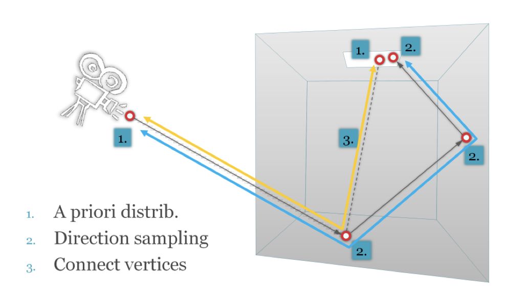
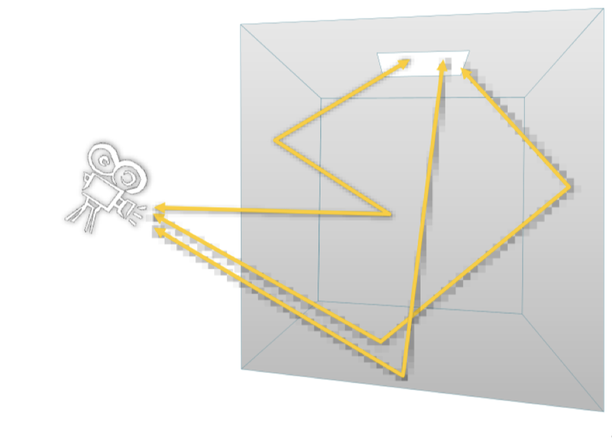
The image above shows a simple path tracer. Along the blue path, we generate the first vertex from the priorly distributed camera surface, and then we pick a random direction form this point such that it passes through the image plane to generate new vertices until the path finally hit the light source. (Operation 2)

You man question how can we guarantee the blue path hit the light source. Actually, we cannot but a light path that do not hit light source contributes nothing to the value so it does not impact the correctness. However, it means there are lots of useless lights calculated, and it results in the waste of time. Thus, we do it in a slightly different way like the yellow path.

Along the yellow path, we use operation 1 to generate a vertex on camera than use operation 2 to generate new vertices. But at the end, we do not expect it to hit the light source. Instead, we use operation 1 to shoot a light from the light source and then apply operation 3 to connect the sub-paths. With this method, we make sure the light path is visible. It is called bidirectional path tracing.

Probability Density Function

By local sampling, we know how to construct a light path. Now we need to evaluate its PDF to calculate the Monte Carlo estimator.

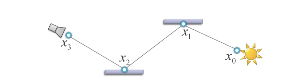
Take the picture above for example. The path PDF can be defined as: \[ p(\bar x) = p(x_0,\cdots,x_3) \] It means the path PDF equals to the joint PDF of path vertices. Applied simple path tracing method the image, then we have: \[ p(x_0,\cdots,x_3) = p(x_3)p(x_2|x_3)p(x_1|x_2)p(x_0) \] Because:

1. \(p(x_3)\): Vertex \(x_3\) comes from a prior distribution over the camera lens that is usually uniform.
2. \(p(x_2|x_3)\): Vertex \(x_2\) is sampled by generating a random direction from \(x_3\), so it is a conditional possibility. Same for \(x_1\).
3. \(p(x_0)\): Sampled from the light source, so it depends on the uniform distribution over the light source. (Recall the bidirectional path tracing mentioned above)

It is not hard to find that the product of these conditional vertex PDFs could the rewritten in a simpler form. \[ p(x_0,\cdots, x_3) = p(x_3)p(x_2)p(x_1)p(x_0) \]

Nonetheless, it is important to keep in mind that the path vertex PDFs for vertices that are not sampled independently are indeed conditional PDFs.

Vertex Sampling

In accordance with the principle of importance sampling, we want to generate full paths paths from a distribution with probability density proportional to the measurement contribution function. That is, high-contribution paths should have proportionally high probability of being sampled. For example, when starting a path on the light source, we usually sample the initial vertex from a distribution proportional to the emitted power. And we usually sample the random direction proportionally to the BRDF at the vertex when extending the path from an existing vertex.

Similarly, when connecting two sub-paths with an edge, we may want to prefer connections with high throughput (though this is rarely done in practice).

Measure Conversion

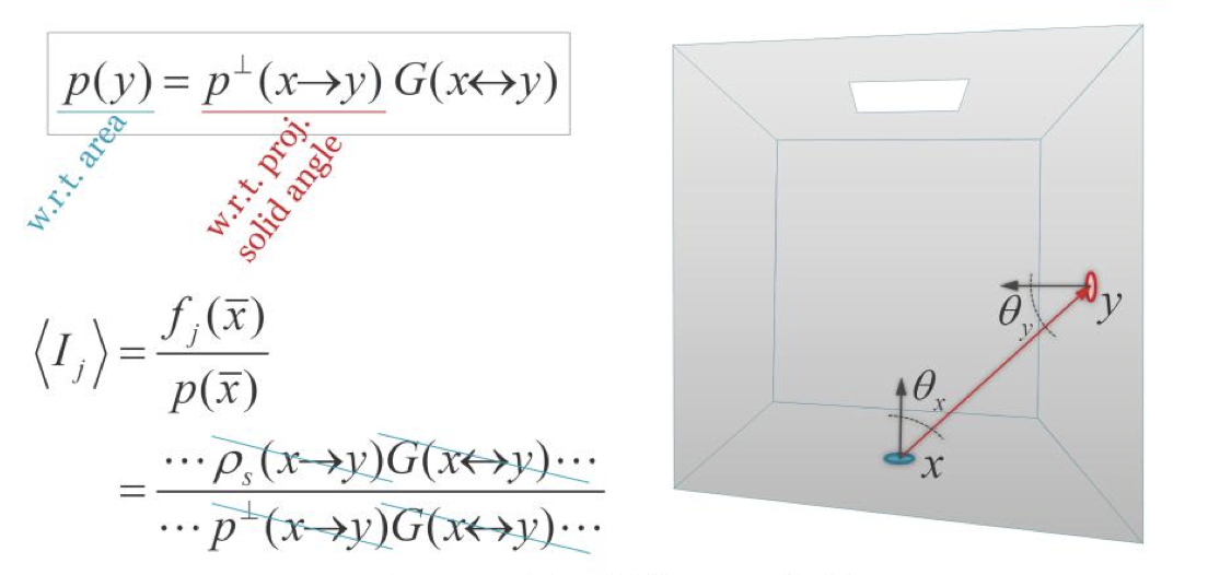
The lecturer mentioned a technical detail of computing the path PDF for vertcies sampled by basic operation 2. As we are integrating the path integral over the surface of the scene, the direction sampling usually gives the PDF with respect to the (projected) solid angle, however.

The conversion factor from the projected solid angle measure to the area measure is the geometry factor. This means that any vertex sampled by shooting a ray along a picked direction has the geometry factor of the generated edge importance sampled.

The only geometry factor that are not importance sampled actually correspond to the connecting edges (operation 3 in local path sampling).

Summary

I think the original lecturer already gives a clear summary about all the contents mentioned above. So that I basically copy paste his points here.

1. The path integral formulation gives the pixel value as an integral over all light transport paths of all lengths.
2. A light transport path is the trajectory of a light carrying particle. It is usually a polyline specified by its vertices.
3. The integrand is the measurement contribution function, which is the product of emitted radiance, sensor sensitivity, and path throughput.
4. Path throughput is the product of BRDFs at the inner path vertices and geometry factors at the path edges.
5. To evaluate the integral, we use Monte Carlo estimator in the form shown at the top right of the slide.
6. To evaluate the estimator, we need to sample a random path from a suitable distribution with PDF p(x).
7. We usually use local path sampling to construct the paths, where we add one vertex at a time. In this case, the full path PDF is given by the product of the (conditional) PDFs for sampling the individual path vertices.

And the conclusion in my words is:

Because of the contradiction between the infinite light paths and finite time and computation resources, a estimating method to simulate the process is necessary. Monte Carlo is a simple unbiased estimation for this purpose.

It's the end of the brief introduction, I hope you understand better why we use Monte Carlo method. And remember, considering the computational cost, path tracing is still an unresolved problem yet.